blood_analysis
blood_analysis.RmdLoad package and data
library(FateMapper)
load(system.file("extdata", "blood_csc.rda", package = "FateMapper"))
Data introduction
The blood lineage tracing dataset is represented as a dataframe with four columns. Each row in the dataset corresponds to a single cell, where the first and second columns contain the embedding information extracted from scRNA-seq data. The third column provides the cell-related barcode derived from lineage tracing data. Lastly, the fourth column represents the annotated cell type of each cell.
head(cell_fate)
#>                           DC_1        DC_2 barcodes celltype
#> CLP_AAACCCACAAAGGGCT -2.038864 -0.20265869        A      CLP
#> CLP_AAACGAACATCCGCGA -1.500590 -0.07898276        1      CLP
#> CLP_AAACGAATCAAGTCTG -1.450054 -0.03668697  1234569      CLP
#> CLP_AAACGCTGTACCGGCT -1.429273 -0.05674879        1      CLP
#> CLP_AAACGCTGTTATCTGG -2.466002 -0.25670260        9      CLP
#> CLP_AAAGAACCATACTGTG -1.056272  0.01399053  12345HG      CLP
clone profile
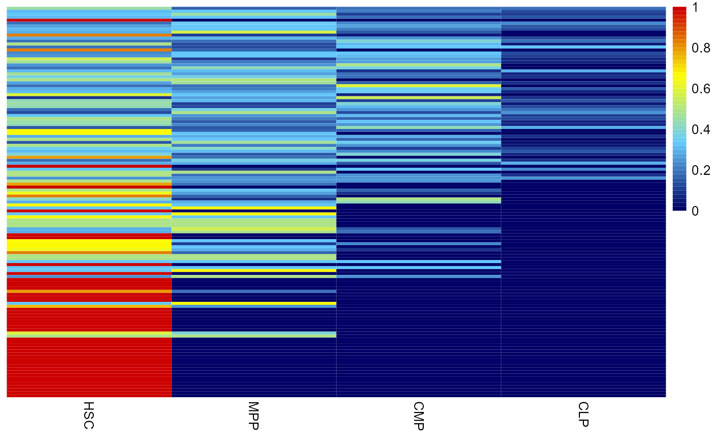
Firstly, we map the clone expression in pseudo-bulk cell types through fate_mapping() function
barcode_freq = fate_mapping(cell_fate,show_row = F,cluster_cols = F,order_use =
                              c('HSC','MPP','CMP','CLP'))
cell type similarity analysis based on clone expression
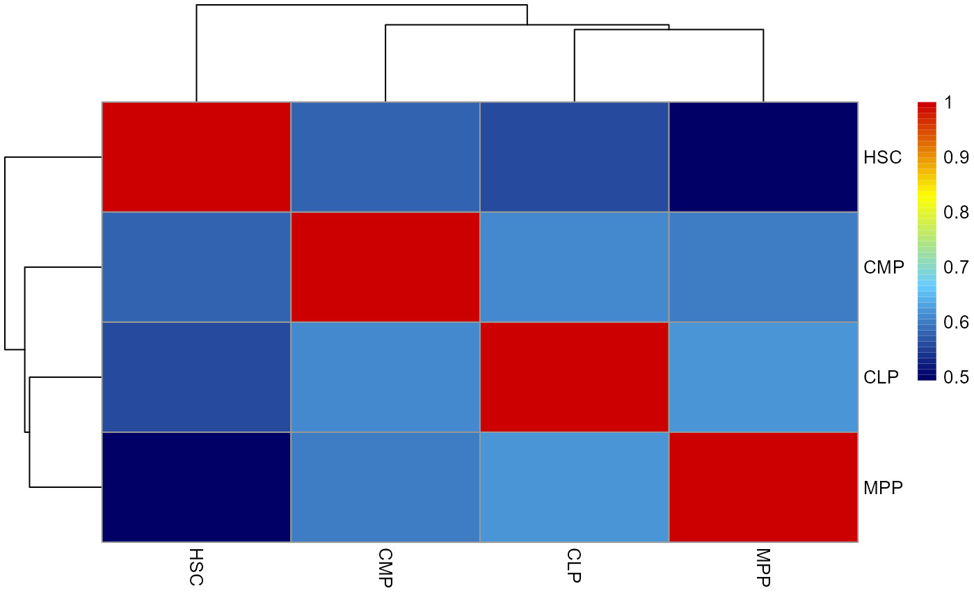
Next, we calculate the spearman correlation between each cell type based on clone expression to estimate the lineage relationships between cell types.
ct_similarity = cell_type_fate_similartiy(cell_fate[,3:4])
Building lineage tree
Building lineage tree based on neighbor-joining method.
lineage_tree(cell_fate[,3:4])
#> Using sample_similarity as value column: use value.var to override.
Clone fate bias analysis
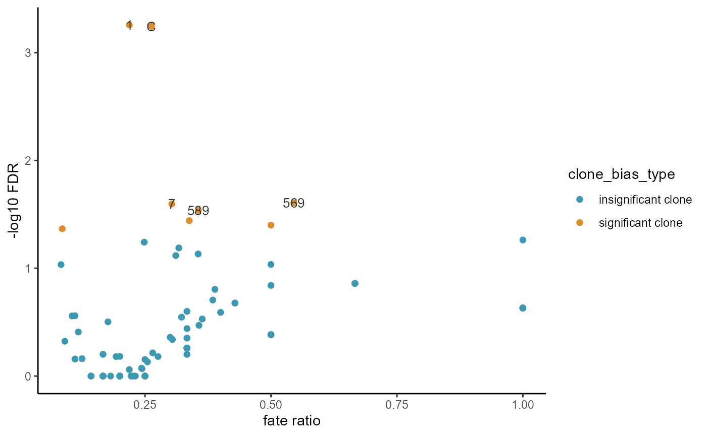
Then, we calculate the clone fate bias based on Fisher-Exact test. Fate bias represent which fate/cell_type the clone is enriched for (e.g. Which cell type does this clone mainly develop into). In this analysis we calculate the clone fate bias for CMP
CMP_bias = clone_fate_bias(cell_fate[,3:4],fate_use = 'CMP')
head(CMP_bias)
#>      clone_name fate_use clone_size        fate_ratio               pvalue
#> X1            1      CMP       1380 0.218840579710145 0.000552808822115242
#> C             C      CMP        643 0.262830482115086 0.000569016009398279
#> X569        569      CMP         11 0.545454545454545   0.0246961006377305
#> X7            7      CMP        155 0.303225806451613     0.02531766742626
#> X589        589      CMP         59 0.355932203389831   0.0289961604540024
#> X12C        12C      CMP         74 0.337837837837838   0.0361563061940716
#>                       fdr
#> X1   0.000552808822115242
#> C    0.000569016009398279
#> X569   0.0246961006377305
#> X7       0.02531766742626
#> X589   0.0289961604540024
#> X12C   0.0361563061940716
fate_bias_summary(CMP_bias)
Clone embedding
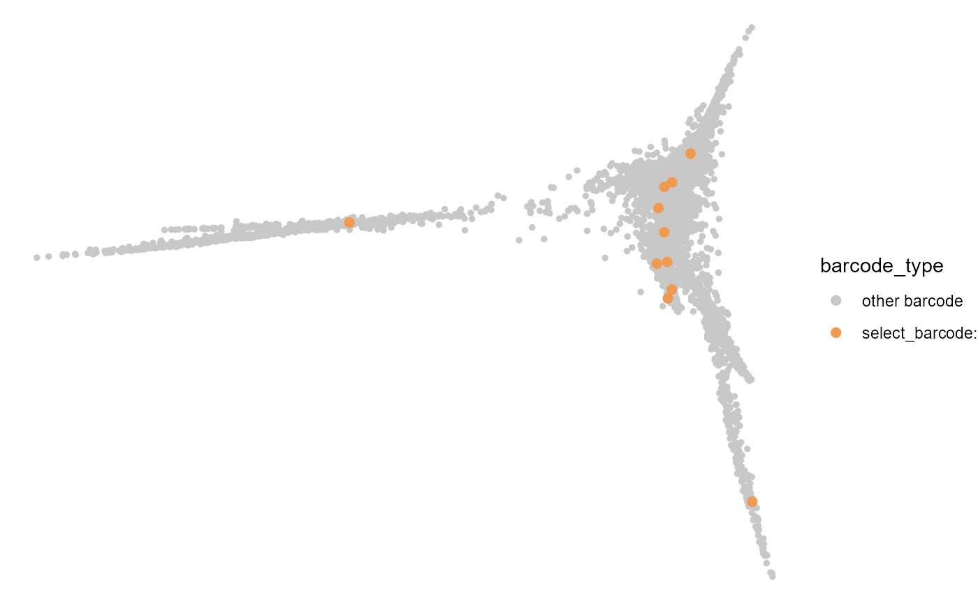
Then we visualize the CMP bias clone on the embedding plot
plot_clone_embedding(CMP_bias[3,1],cell_fate,colors = c(rgb(200/255,200/255,200/255),
                                             rgb(239/255,153/255,81/255)))